refer to table 15-4. what is shaktis profit-maximizing output?
Learning Objectives
- Depict how a monopolistic competitor chooses price and quantity using marginal revenue and marginal toll
- Graph and translate a monopolistically competitive firm's average, marginal, and total cost curves
- Compute full acquirement, profits, and losses for monopolistic competitors using the demand and average cost curves
Choosing the Profit-Maximizing Output and Price
The monopolistically competitive house decides on its turn a profit-maximizing quantity and toll in much the same manner as a monopolist. A monopolistic competitor, like a monopolist, faces a downward-sloping demand bend, and so information technology will cull some combination of cost and quantity along its perceived demand bend.
Equally an example of a turn a profit-maximizing monopolistic competitor, consider the Accurate Chinese Pizza store, which serves pizza with cheese, sugariness and sour sauce, and your choice of vegetables and meats. Although Authentic Chinese Pizza must compete against other pizza businesses and restaurants, it has a differentiated product. The house'due south perceived demand curve is downward sloping, equally shown in Figure 1 and the first 2 columns of Table ane.
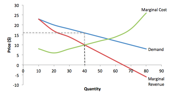
Figure 1. How a Monopolistic Competitor Chooses its Turn a profit Maximizing Output and Price. To maximize profits, the Accurate Chinese Pizza shop would choose a quantity where marginal revenue equals marginal cost, or Q where MR = MC. Hither it would choose a quantity of forty and a cost of $16.
| Table 1. Revenue and Cost Schedule | |||||
|---|---|---|---|---|---|
| Quantity | Price | Total Revenue | Marginal Revenue | Total Price | Marginal Price |
| ten | $23 | $230 | — | $340 | – |
| xx | $20 | $400 | $17 | $400 | $6 |
| thirty | $18 | $540 | $14 | $480 | $viii |
| 40 | $16 | $640 | $10 | $580 | $10 |
| 50 | $xiv | $700 | $half-dozen | $700 | $12 |
| threescore | $12 | $720 | $2 | $840 | $fourteen |
| seventy | $x | $700 | –$2 | $ane,020 | $18 |
| 80 | $8 | $640 | –$6 | $1,280 | $26 |
The combinations of price and quantity at each point on the demand curve tin can be multiplied to calculate the total revenue that the firm would receive, which is shown in the tertiary column of Tabular array 1. The fourth cavalcade, marginal revenue, is calculated every bit the change in total revenue divided past the change in quantity. The final columns of Tabular array i show total cost, marginal cost, and boilerplate cost. As always, marginal cost is calculated by dividing the alter in full price by the change in quantity, while boilerplate price is calculated by dividing full toll by quantity. The following example shows how these firms calculate how much of its production to supply at what toll.
How a Monopolistic Competitor Determines How Much to Produce and at What Toll
The procedure by which a monopolistic competitor chooses its turn a profit-maximizing quantity and cost resembles closely how a monopoly makes these decisions procedure. Outset, the house selects the profit-maximizing quantity to produce. Then the business firm decides what cost to charge for that quantity.
Step ane. The monopolistic competitor determines its turn a profit-maximizing level of output. In this instance, the Accurate Chinese Pizza company volition determine the profit-maximizing quantity to produce by considering its marginal revenues and marginal costs. Two scenarios are possible:
- If the firm is producing at a quantity of output where marginal revenue exceeds marginal cost, and then the firm should proceed expanding product, because each marginal unit is adding to profit by bringing in more than acquirement than its price. In this manner, the business firm will produce up to the quantity where MR = MC.
- If the business firm is producing at a quantity where marginal costs exceed marginal revenue, and so each marginal unit is costing more than than the revenue it brings in, and the business firm will increase its profits by reducing the quantity of output until MR = MC.
In this example, MR and MC intersect at a quantity of 40, which is the turn a profit-maximizing level of output for the firm.
Step two. The monopolistic competitor decides what price to charge. When the firm has determined its profit-maximizing quantity of output, it can then look to its perceived need bend to notice out what information technology tin charge for that quantity of output. On the graph, this process can be shown as a vertical line reaching up through the profit-maximizing quantity until it hits the house's perceived demand bend. For Authentic Chinese Pizza, information technology should accuse a price of $xvi per pizza for a quantity of twoscore.
Although the process by which a monopolistic competitor makes decisions about quantity and price is similar to the fashion in which a monopolist makes such decisions, two differences are worth remembering. First, although both a monopolist and a monopolistic competitor face downwards-sloping demand curves, the monopolist's perceived demand bend is the market demand curve, while the perceived need curve for a monopolistic competitor is based on the extent of its product differentiation and how many competitors it faces. Second, a monopolist is surrounded by barriers to entry and need not fright entry, but a monopolistic competitor who earns profits must expect the entry of firms with like, but differentiated, products.
Try Information technology
Calculating Profits
Once the monopollstic competitor has determined the profit-maximizing quantity of output to supply, the adjacent step is to calculate how much profit it is earning. We use the same process that was used with perfect competition and monopoly. This is illustrated in Figure 2, using the data from Table 2, which extends the information from to Table 1 to include average total cost in the last column.
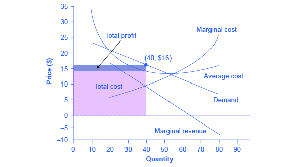
Figure 2. Computing Turn a profit for a Monopolistic Competitor. To calculate profit, start from the turn a profit-maximizing quantity, which is 40. Next find total revenue which is the area of the rectangle with the elevation of P = $16 times the base of Q = 40. Adjacent discover full price which is the area of the rectangle with the height of Ac = $14.50 times the base of Q = 40. The difference betwixt the two areas is turn a profit, the small rectangle to a higher place full cost in the effigy.
| Tabular array 2. Revenue and Cost Schedule, including Boilerplate Price | ||||||
|---|---|---|---|---|---|---|
| Quantity | Price | Total Revenue | Marginal Acquirement | Total Cost | Marginal Cost | Average Cost |
| 10 | $23 | $230 | — | $340 | – | $34 |
| xx | $20 | $400 | $17 | $400 | $6 | $20 |
| xxx | $18 | $540 | $14 | $480 | $8 | $16 |
| 40 | $16 | $640 | $10 | $580 | $10 | $fourteen.50 |
| 50 | $xiv | $700 | $6 | $700 | $12 | $14 |
| sixty | $12 | $720 | $2 | $840 | $fourteen | $14 |
| seventy | $ten | $700 | –$2 | $1,020 | $xviii | $14.57 |
| 80 | $viii | $640 | –$half dozen | $1,280 | $26 | $16 |
Nosotros showtime by identifying the turn a profit-maximizing level of output, where marginal revenue equals marginal cost. This is Q = xl. Adjacent, wait for the profit margin, the difference betwixt toll and average toll. The cost is $sixteen, which you lot can read off the demand curve for quantity equals 40. The average cost is $14.50, which you lot tin can read off the average cost curve for quantity equals 40. The profit margin is $16.00 – $14.50 = $i.50 for each unit that the firm sells. Total profit is the profit margin times the quantity or $i.50 x forty = $60.
Alternatively, we tin can compute profit as total revenue minus total cost. Total revenue is price times quantity or $xvi.00 x twoscore = $640. This is the area of the rectangle that starts at the origin, goes up to a price of $16, goes over to the demand curve, down to the quantity of 40 and back to the origin. Total cost is average cost times quantity or $14.fifty ten 40 = $580. This is the surface area of the rectangle that starts at the origin, goes up the vertical axis to an average cost of $14.50, goes over to the average toll curve, down to the quantity of 40 and back to the origin. Profit is the difference between the two areas, $640 – $580 = $threescore. This is shown graphically as the area of the rectangle on top of total cost, or the price minus average cost, times quantity. Note that if the firm was earning zero economical profits, the rectangles of total revenue and total cost would exist the aforementioned—in that location would exist no turn a profit rectangle. The pause-fifty-fifty point occurs where the demand curve intersects with average toll, so P = AC. Annotation also that if the firm was making a loss, the negative profit (i.e. loss) would be the rectangle on top of total acquirement.
Try It
Contribute!
Did yous accept an idea for improving this content? Nosotros'd love your input.
Improve this pageLearn More
Source: https://courses.lumenlearning.com/wm-microeconomics/chapter/profit-maximization-under-monopolistic-competition/
0 Response to "refer to table 15-4. what is shaktis profit-maximizing output?"
Post a Comment